Chapter 11 External validity and inference aggregation

11.1 Transportation of findings across contexts

Say we study the effect of \(X\) on \(Y\) in case 0 (a country, for instance) and want to make inferences to case 1 (another country). Our problem however is that effects are heterogeneous and features that differ across units may be related both to treatment assignment, outcomes, and selection into the sample. This is the problem studied by Pearl and Bareinboim (2014). In particular Pearl and Bareinboim (2014) show for which nodes data is needed in order to “licence” external claims, given a model.

We illustrate with a simple model in which a confounder has a different distribution in a study site and a target site.

model <- make_model("Case -> W  -> X -> Y <- W") %>%
  set_restrictions("W[Case = 1] < W[Case = 0]") %>%
  set_parameters(node = "X", statement = "X[W=1]>X[W=0]", parameters = 1/2)%>%
  set_parameters(node = "Y", statement = complements("W", "X", "Y"), parameters = .17) %>%
  set_parameters(node = "Y", statement = decreasing("X", "Y"), parameters = 0) 
model$parameters_df

##    param_names param_value param_set node nodal_type
## 1       Case.0     0.50000      Case Case          0
## 2       Case.1     0.50000      Case Case          1
## 3         W.00     0.33333         W    W         00
## 4         W.01     0.33333         W    W         01
## 5         W.11     0.33333         W    W         11
## 6         X.00     0.16667         X    X         00
## 7         X.10     0.16667         X    X         10
## 8         X.01     0.50000         X    X         01
## 9         X.11     0.16667         X    X         11
## 10      Y.0000     0.03132         Y    Y       0000
## 11      Y.1000     0.00000         Y    Y       1000
## 12      Y.0100     0.00000         Y    Y       0100
## 13      Y.1100     0.00000         Y    Y       1100
## 14      Y.0010     0.03132         Y    Y       0010
## 15      Y.1010     0.03132         Y    Y       1010
## 16      Y.0110     0.00000         Y    Y       0110
## 17      Y.1110     0.00000         Y    Y       1110
## 18      Y.0001     0.39040         Y    Y       0001
## 19      Y.1001     0.00000         Y    Y       1001
## 20      Y.0101     0.03132         Y    Y       0101
## 21      Y.1101     0.00000         Y    Y       1101
## 22      Y.0011     0.03132         Y    Y       0011
## 23      Y.1011     0.39040         Y    Y       1011
## 24      Y.0111     0.03132         Y    Y       0111
## 25      Y.1111     0.03132         Y    Y       1111
##    gen priors
## 1    1      1
## 2    1      1
## 3    2      1
## 4    2      1
## 5    2      1
## 6    3      1
## 7    3      1
## 8    3      1
## 9    3      1
## 10   4      1
## 11   4      1
## 12   4      1
## 13   4      1
## 14   4      1
## 15   4      1
## 16   4      1
## 17   4      1
## 18   4      1
## 19   4      1
## 20   4      1
## 21   4      1
## 22   4      1
## 23   4      1
## 24   4      1
## 25   4      1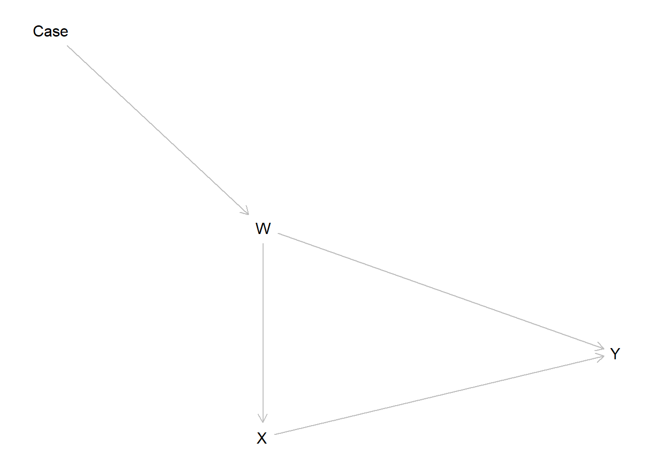

plot(model)

We start by checking some basic quantities in the priors and the posteriors, we will then see how we do with data.

query_model(model,
            queries = list(Incidence = "W==1", 
                           ATE = "Y[X=1] - Y[X=0]", 
                           CATE = "Y[X=1, W=1] - Y[X=0, W=1]"),
            given = c("Case==0", "Case==1"),
            using = c("priors", "parameters"), expand_grid = TRUE) %>% kable

Query	Given	Using	mean	sd
Incidence	Case==0	priors	0.339	0.234
Incidence	Case==0	parameters	0.333
Incidence	Case==1	priors	0.666	0.235
Incidence	Case==1	parameters	0.667
ATE	Case==0	priors	0.002	0.139
ATE	Case==0	parameters	0.333
ATE	Case==1	priors	0.001	0.139
ATE	Case==1	parameters	0.573
CATE	Case==0	priors	0.000	0.169
CATE	Case==0	parameters	0.812
CATE	Case==1	priors	0.000	0.169
CATE	Case==1	parameters	0.812

We see that the incidence of \(W\) as well as the ATE of \(X\) on \(Y\) is larger in case 1 than in case 0 (in parameters, though not in priors). However the effect of \(X\) on \(Y\) conditional on \(W\) is the same in both places.

We now update the model using data on \(X\) and \(Y\) only from one case (case 1) and data on W from both and check inferences on the other.

The function make_data lets us generate data like this by specifying a multistage data strategy:

data <- make_data(model, n = 1000, 
                  vars = list(c("Case", "W"), c("X", "Y")), 
                  probs = c(1,1),
                  subsets = c(TRUE, "Case ==1"))

transport <- update_model(model, data)

query_model(transport,
            queries = list(Incidence = "W==1", 
                           ATE = "Y[X=1] - Y[X=0]", 
                           CATE = "Y[X=1, W=1] - Y[X=0, W=1]"),
            given = c("Case==0", "Case==1"),
            using = c("posteriors", "parameters"), expand_grid = TRUE)

Table 11.1: Extrapolation when two sites differ on \(W\) and \(W\) is observable in both sites
Query	Given	Using	mean	sd
Incidence	Case==0	posteriors	0.336	0.007
Incidence	Case==0	parameters	0.333
Incidence	Case==1	posteriors	0.661	0.007
Incidence	Case==1	parameters	0.667
ATE	Case==0	posteriors	0.340	0.011
ATE	Case==0	parameters	0.333
ATE	Case==1	posteriors	0.570	0.009
ATE	Case==1	parameters	0.573
CATE	Case==0	posteriors	0.810	0.009
CATE	Case==0	parameters	0.812
CATE	Case==1	posteriors	0.810	0.009
CATE	Case==1	parameters	0.812

We do well in recovering the (different) effects both in the location we study and the one in which we do not. In essence querying the model for the out of sample case requests a type of post stratification. We get the right answer, though as always this depends on the model being correct.

Had we attempted to make the extrapolation without data on \(W\) in country 1 we would get it wrong. In that case however we would also report greater posterior variance. The posterior variance here captures the fact that we know things could be different in country 1, but we don’t know in what way they are different. Note that we get the CATE right since in the model this is assumed to be the same across cases.

Table 11.2: Extrapolation when two sites differ on \(W\) and \(W\) is not observable in target country.
Query	Given	Using	mean	sd
Incidence	Case==0	posteriors	0.329	0.007
Incidence	Case==0	parameters	0.333
Incidence	Case==1	posteriors	0.675	0.007
Incidence	Case==1	parameters	0.667
ATE	Case==0	posteriors	0.319	0.011
ATE	Case==0	parameters	0.333
ATE	Case==1	posteriors	0.572	0.009
ATE	Case==1	parameters	0.573
CATE	Case==0	posteriors	0.811	0.009
CATE	Case==0	parameters	0.812
CATE	Case==1	posteriors	0.811	0.009
CATE	Case==1	parameters	0.812

11.2 Combining observational and experimental data

An interesting weakness of experimental studies is that, by dealing so effectively with self selection into treatment, they limit our ability to learn about self selection. Often however we want to know what causal effects would be specifically for people that would take up a treatment in non experimental settings. This kind of problem is studied for example by by Knox et al. (2019).

A causal model can encompass both experimental and observational data and let you answer this kind of question. To illustrate, imagine that node \(R\) indicates whether a unit was assigned to be randomly assigned to treatment assignment (\(X=Z\) if \(R=1\)) or took on its observational value (\(X=O\) if \(R=0\)). We assume the exclusion restriction that entering the experimental sample is not related to \(Y\) other than through assignment of \(X\).

model <- make_model("R -> X -> Y; O -> X <- Z; O <-> Y") %>%
  
    set_restrictions("(X[R=1, Z=0]!=0) | (X[R=1, Z=1]!=1) | (X[R=0, O=0]!=0) | (X[R=0, O=1]!=1)")

plot(model)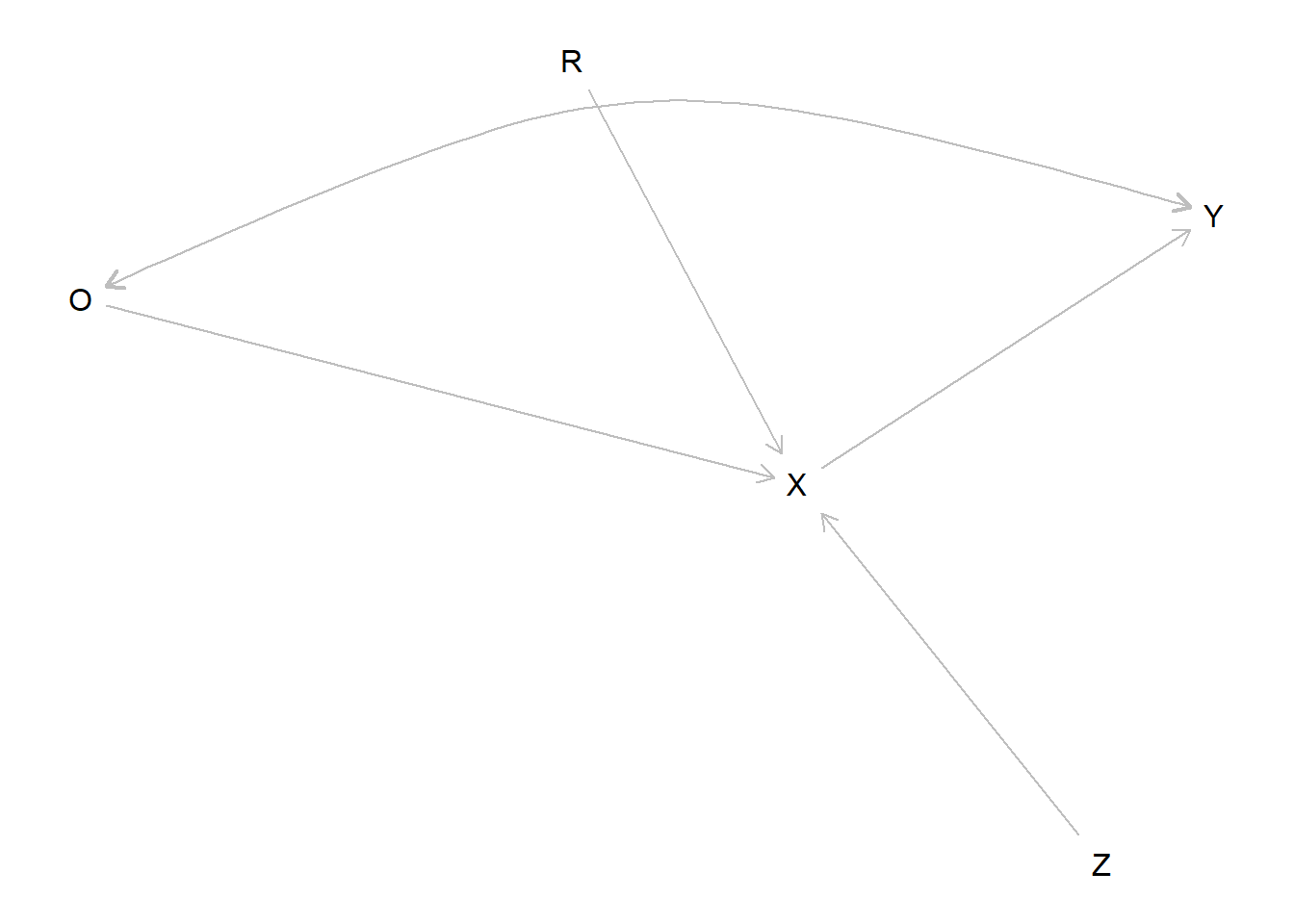

The parameter matrix has just one type for \(X\) since \(X\) really operates here as a kind of switch, inheriting the value of \(Z\) or \(O\) depending on \(R\). Parameters allow for complete confounding between \(O\) and \(Y\) but \(Z\) and \(Y\) are unconfounded.

We imagine parameter values in which there is a true .2 effect of \(X\) on \(Y\). However the effect is positive (.4) for cases in which \(X=1\) under observational assignment but negative (-.2) for cases in which \(X=0\) under observational assignment.

model <- model %>%
    set_parameters(node = "Y", confound = "O==0", parameters = c(.8, .2,  0,  0)) %>%
    set_parameters(node = "Y", confound = "O==1", parameters = c( 0,  0, .6, .4))

To parse this expression: we allow different parameter values for the four possible nodal types for \(Y\) when \(O=0\) and when \(O=1\). When \(O=0\) we have \((\lambda_{00} = .8, \lambda_{10} = .2, \lambda_{01} = 0, \lambda_{11} = 0)\) which implies a negative treatment effect and many \(Y=0\) observations. When \(O=1\) we have \((\lambda_{00} = 0, \lambda_{10} = 0, \lambda_{01} = .6, \lambda_{11} = .4)\) which implies a positive treatment effect and many \(Y=1\) observations.

The estimands:

Table 11.3: estimands
Query	Given	Using	mean
ATE	-	parameters	0.2
ATE	R==0	parameters	0.2
ATE	R==1	parameters	0.2

The priors:

Table 11.4: priors
Query	Given	Using	mean	sd
ATE	-	priors	-0.002	0.257
ATE	R==0	priors	-0.002	0.257
ATE	R==1	priors	-0.002	0.257

Data:

data <- make_data(model, n = 800)

The true effect is .2 but naive analysis on the observational data would yield a strongly upwardly biased estimate.

estimatr::difference_in_means(Y~X, data = filter(data, R==0))

Table 11.5: Inferences on the ATE from differences in means
	Estimate	Std. Error	t value	Pr(>\|t\|)	CI Lower	CI Upper	DF
X	0.743	0.033	22.69	0	0.678	0.808	178

The CausalQueries estimates are:

posterior <- update_model(model, data)

Query	Given	Using	mean	sd
ATE	-	posteriors	0.203	0.031
ATE	R==0	posteriors	0.203	0.031
ATE	R==1	posteriors	0.203	0.031

Much better.

This model used both the experimental and the observational data. It is interesting to ask whether the observational data improved the estimates from the experimental data or did everything depend on the experimental data?

To see, lets do updating using experimental data only:

updated_no_O <- update_model(model, dplyr::filter(data, R==1))

Query	Given	Using	mean	sd
ATE	-	posteriors	0.24	0.035
ATE	R==0	posteriors	0.24	0.035
ATE	R==1	posteriors	0.24	0.035

In this case we get a tightening of posterior variance and a more accurate result when we use the observational data but the gains are relatively small. They would be smaller still if we had more data, in which case inferences from the experimental data would be more accurate still.

In both cases the estimates for the average effect in the randomized and the observationally assigned group are the same. This is how it should be since these are, afterall, randomly assigned into these groups.

Heterogeneity in this model lies between those that are in treatment and those that are in control in the observational sample. We learn nothing about this heterogeneity from the experimental data alone but we learn a lot from the mixed model, picking up the strong self selection into treatment in the observational group:

Query	Given	Using	mean	sd
ATE	R==1 & X==0	posteriors	0.203	0.031
ATE	R==1 & X==1	posteriors	0.203	0.031
ATE	R==0 & X==0	posteriors	-0.183	0.027
ATE	R==0 & X==1	posteriors	0.593	0.048

11.3 A jigsaw puzzle: Learning across populations

Consider a situation in which we believe the same model holds in multiple sites but in which learning about the model requires combining data about different parts of the model from multiple studies.

model <- make_model("X -> Y <- Z -> K") %>%

          set_parameters(
            statement = list("(Y[X=1, Z = 1] > Y[X=0, Z = 1])",  
                             "(K[Z = 1] > K[Z = 0])"),
            node = c("Y","K"), 
            parameters = c(.24,.85))

plot(model)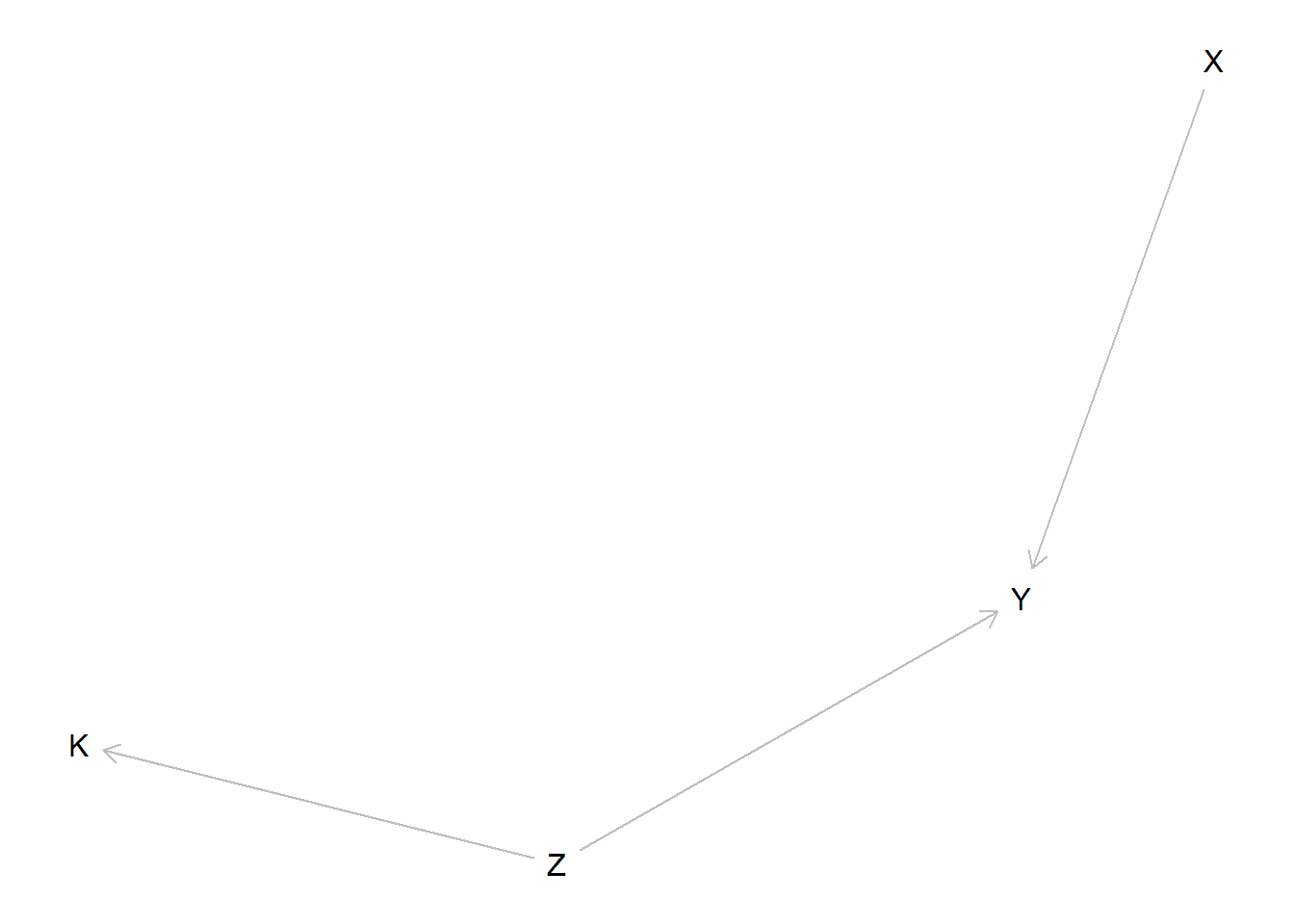

We imagine we have access to three types of data;

Study 1 is an experiment looking at the effects of \(X\) on \(Y\), ancillary data on context, \(K\) is collected but \(Z\) is not observed
Study 2 is a factorial study examining the joint effects of \(X\) and \(Z\) on \(Y\), \(K\) is not observed
Study 3 is an RCT looking at the relation between \(Z\) and \(K\). \(X\) and \(Y\) are not observed.

df <- make_data(model, 300, using = "parameters") %>%
  
      mutate(study = rep(1:3, each = 100),
             K = ifelse(study == 1, NA, K),
             X = ifelse(study == 2, NA, X),
             Y = ifelse(study == 2, NA, Y),
             Z = ifelse(study == 3, NA, Z)
             )

Tables 11.6 - 11.8 show conditional inferences for the probability that \(X\) caused \(Y\) in \(X=Y=1\) cases conditional on \(K\) for each study, analyzed individually

Table 11.6: Clue is uninformative in Study 1
Given	mean	sd
X == 1 & Y == 1 & K == 1	0.501	0.165
X == 1 & Y == 1 & K == 0	0.502	0.162

Table 11.7: Clue is also uninformative in Study 2 (factorial)
Given	mean	sd
X == 1 & Y == 1 & K == 1	0.530	0.123
X == 1 & Y == 1 & K == 0	0.529	0.121

Table 11.8: Clue is also uninformative in Study 3 (experiment studying \(K\))
Given	mean	sd
X == 1 & Y == 1 & K == 1	0.503	0.161
X == 1 & Y == 1 & K == 0	0.502	0.161

In no case is \(K\) informative. In study 1 data on \(K\) is not available, in study 2 it is available but researchers do not know, quantitatively, how it relates to \(Z\). In the third study the \(Z,K\) relationship is well understood but the joint relation between \(Z,X\), and \(Y\) is not understood.

Table 11.9 shows the inferences when the data are combined with joint updating across all parameters.

Table 11.9: Clue is informative after combining studies linking \(K\) to \(Z\) and \(Z\) to \(Y\)
Given	mean	sd
X == 1 & Y == 1 & K == 1	0.760	0.085
X == 1 & Y == 1 & K == 0	0.493	0.066
X == 1 & Y == 1 & K == 1 & Z == 1	0.799	0.094
X == 1 & Y == 1 & K == 0 & Z == 1	0.799	0.094
X == 1 & Y == 1 & K == 1 & Z == 0	0.488	0.067
X == 1 & Y == 1 & K == 0 & Z == 0	0.488	0.067

Here fuller understanding of the model lets researchers use information on \(Z\) to update on values for \(Z\) and in turn update on the likely effects of \(X\) on \(Y\). Rows 3-6 highlight that the updating works through inferences on \(Z\) and there are no gains when \(Z\) is known, as in Study 2.

The collection of studies collectively allow for inferences that are not possible from any one study.

References

Knox, Dean, Teppei Yamamoto, Matthew A Baum, and Adam J Berinsky. 2019. “Design, Identification, and Sensitivity Analysis for Patient Preference Trials.” Journal of the American Statistical Association, 1–27.

Pearl, Judea, and Elias Bareinboim. 2014. “External Validity: From Do-Calculus to Transportability Across Populations.” Statistical Science 29 (4): 579–95.