Part 2 Design steps
2.1 Population
The challenge is to generate a population with members that belong to the hidden and non-hidden populations, but that also have membership (or not) in some other group. The population must have a networks structure that reflects plausible types of in-group and out-group connections for each of these groups. This is implemented with the get_study_population() function in the package.
The first step is to draw a simulated population. This is done using the function get_study_population(). Using default parameters we can draw one simulation of population of size \(2000\) as follows:
| name | 1 | 2 | 3 | 4 | 5 | 6 |
| known | 0 | 0 | 0 | 0 | 0 | 0 |
| hidden | 0 | 0 | 0 | 0 | 0 | 0 |
| type | 00 | 00 | 00 | 00 | 00 | 00 |
| p_visibility_known | 1 | 1 | 1 | 1 | 1 | 1 |
| known_visible | 2 | 1 | 2 | 1 | 3 | 1 |
| p_visibility_hidden | 0.685 | 0.726 | 0.627 | 0.628 | 0.762 | 0.731 |
| hidden_visible | 0 | 0 | 2 | 0 | 0 | 1 |
| type_visible_00 | 4 | 2 | 1 | 3 | 2 | 1 |
| type_visible_01 | 0 | 0 | 0 | 0 | 0 | 1 |
| type_visible_10 | 2 | 1 | 0 | 1 | 3 | 1 |
| type_visible_11 | 0 | 0 | 2 | 0 | 0 | 0 |
| n_visible | 6 | 3 | 3 | 4 | 5 | 3 |
| links | c(73, 215, 682, 1252, 1380, 1486) | c(893, 899, 1420) | c(770, 1948, 1993) | c(107, 113, 1239, 1353) | c(103, 144, 1424, 1637, 1685) | c(299, 1478, 1810) |
| total | 2000 | 2000 | 2000 | 2000 | 2000 | 2000 |
| service_use | 0 | 1 | 0 | 0 | 1 | 1 |
| loc_1 | 0 | 0 | 0 | 1 | 0 | 0 |
| loc_2 | 0 | 0 | 0 | 0 | 0 | 0 |
| loc_3 | 0 | 0 | 0 | 0 | 0 | 0 |
| known_2 | 0 | 0 | 0 | 0 | 0 | 0 |
| known_3 | 0 | 0 | 0 | 0 | 0 | 0 |
| total_known | 625 | 625 | 625 | 625 | 625 | 625 |
| total_hidden | 197 | 197 | 197 | 197 | 197 | 197 |
| total_service_use | 591 | 591 | 591 | 591 | 591 | 591 |
| total_loc_1 | 555 | 555 | 555 | 555 | 555 | 555 |
| total_loc_2 | 208 | 208 | 208 | 208 | 208 | 208 |
| total_loc_3 | 455 | 455 | 455 | 455 | 455 | 455 |
| total_known_2 | 191 | 191 | 191 | 191 | 191 | 191 |
| total_known_3 | 402 | 402 | 402 | 402 | 402 | 402 |
| service_use_visible | 1 | 0 | 0 | 2 | 3 | 1 |
| loc_1_visible | 1 | 2 | 1 | 1 | 0 | 2 |
| loc_2_visible | 1 | 0 | 0 | 0 | 0 | 0 |
| loc_3_visible | 1 | 0 | 0 | 1 | 2 | 2 |
| known_2_visible | 1 | 0 | 0 | 0 | 0 | 1 |
| known_3_visible | 3 | 1 | 1 | 1 | 1 | 1 |
2.1.1 Population Parameters
Full details on parameters are provided in the package documentation (via ?). See also section ??.
The key parameters you can provide to the population function are:
N– size of populationK– number of groups (with \(M < K\) such that groups \(K - M, \dots, K\) have unknown size). For simplicity we can assume \(K = 2,\, M = 1\)prev_K– prevalence of each group in populationrho_K– correlations in group membershipp_edge_within,p_edge_between– probability of edges within and between groupsp_visibility– average probability of revealing particular group membership relevant for all types of sampling. Essentially this represents whether group membership of individual will be observed by others. In addition, in RDS sampling this parameter affects whether members of hidden group will participate in the study if they are given a couponadd_groups– average probabilities of other binary individual characteristics (e.g. services utilization, time-location presence, group memberships)
These parameters are used to form an adjacency matrix \(G\) (possibly directed underlying graph \((V,E)\)) with \(\mathbf{d}\) representing the vector of individual degrees.
The resulting data frame has one row per person. In addition to network structure the data records the unit’s type (membership in multiple groups).
Below we show an example of simulated population with the following set of parameters:
N = 2000, K = 2, prev_K = c(known = 0.3, hidden = 0.1), rho_K = 0.05, p_edge_within = list(known = c(0.05, 0.05), hidden = c(0.05, 0.9)), p_edge_between = list(known = 0.05, hidden = 0.01), p_visibility = list(hidden = 0.7, known = 0.99), add_groups = list(service_use = 0.3, loc_1 = 0.3, loc_2 = 0.1, loc_3 = 0.2, known_2 = 0.1, known_3 = 0.2)
2.1.2 Example
population_study <-
  do.call(what = declare_population,
          args = c(handler = get_study_population, study_1[1:8]))


set.seed(19872312)
population <- population_study()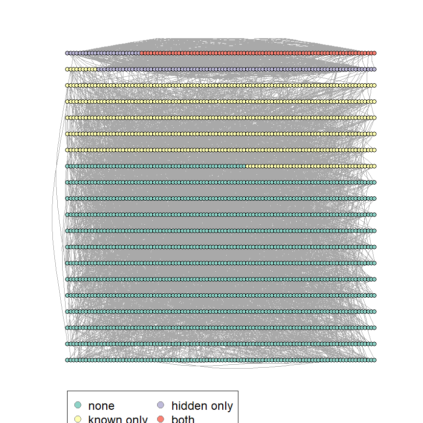
(#fig:study_pop)Population in study 1
2.1.3 Considerations
Things to consider in the future:
- Individuals can have parameters representing barrier effects, transmission and recall biases (Maltiel et al. 2015)
- Using more complex models (e.g. ERGM or block ERGM) to generate the network structure instead of simple block structure used currently
- The propensity to recruit can be dependent on the blocks (membership in groups) (Berchenko, Rosenblatt, and Frost 2017)
2.2 Sampling strategies
2.2.1 RDS Sampling
The RDS function takes the population data frame and then implements a simulated RDS procedure to return a data frame that records whether someone was sampled as well as information about how they were sampled, particularly in which wave and at what time.
For instance:
| name | type | rds | rds_from | rds_t | rds_wave | rds_hidden | rds_own_coupon | rds_coupon_1 | rds_coupon_2 | rds_coupon_3 |
|---|---|---|---|---|---|---|---|---|---|---|
| 1811 | 01 | 1 | 1918 | 32 | 3 | 1 | 9-2-2 | 9-2-2-1 | 9-2-2-2 | 9-2-2-3 |
| 1816 | 01 | 1 | 1955 | 25 | 5 | 1 | 6-3-2-2-3 | 6-3-2-2-3-1 | 6-3-2-2-3-2 | 6-3-2-2-3-3 |
| 1825 | 01 | 1 | 1839 | 27 | 3 | 1 | 3-1-2 | 3-1-2-1 | 3-1-2-2 | 3-1-2-3 |
| 1826 | 01 | 1 | 1852 | 28 | 2 | 1 | 8-3 | 8-3-1 | 8-3-2 | 8-3-3 |
| 1827 | 01 | 1 | 1893 | 34 | 4 | 1 | 6-3-3-2 | 6-3-3-2-1 | 6-3-3-2-2 | 6-3-3-2-3 |
| 1834 | 01 | 1 | 1845 | 19 | 3 | 1 | 6-3-2 | 6-3-2-1 | 6-3-2-2 | 6-3-2-3 |
In RDS sample we need to draw recruitment graph, degrees of recruited individuals, timing of recruitment, coupon matrix and derive \(I_{t}\), number of active recruiters at any stage (presuming that if someone has a non-activated coupon, they are active recruiters), from this data
RDS parameter options:
n_seed– The number of starting seeds from hidden population. Currently these are assumed to be drawn according to simple random sampling.n_coupons– Number of coupons assigned to each seedtarget_type– Whether the sampling aims to enroll particular number of respondents or wavestarget_n_rds– Target sample size or number of waves depending ontarget_type
2.2.2 TLS Sampling
The TLS function takes the population data frame and then implements a mapping of locations, samples locations, and samples individuals in those locations.
For instance:
population <- get_study_population(
  N = 1000,
  add_groups = list(p_service = 0.3, loc_1 = .1, loc_2 = .2, loc_3 = .3))

sample <- sample_tls(population)| name | hidden | tls_loc_sampled | tls |
|---|---|---|---|
| 890 | 1 | loc_3 | 1 |
| 892 | 1 | loc_2 | 1 |
| 894 | 1 | loc_3 | 1 |
| 895 | 1 | loc_2 | 1 |
| 897 | 1 | loc_3 | 1 |
| 901 | 1 | loc_3 | 1 |
2.2.3 PPS Sampling
The PPS function takes the population data and samples individuals proportionally to the size of strata defined by their group memberships
For instance:
| name | hidden | pps_share | pps |
|---|---|---|---|
| 2 | 0 | 0.484 | 1 |
| 5 | 0 | 0.484 | 1 |
| 6 | 0 | 0.484 | 1 |
| 7 | 0 | 0.484 | 1 |
| 9 | 0 | 0.484 | 1 |
| 14 | 0 | 0.484 | 1 |
2.2.4 Considerations
For NSUM we also need a proportional sample from the population with the same data structure except we do not need timing and coupon matrices
For Service Multiplier we need data on participation in target program within RDS sample. In addition we need an estimate of total hidden population program participation
How the seeds in RDS selected? Do we specifically target connected individuals (to increase chances of enrollment) or individuals with varying degrees (to increase sample coverage)?
Can RDS enroll non-target population?
Are individuals with less than
n_couponslinks allowed to enter study?What happens if sampling stops prior to the target size/waves? Do we allow enrollment of more seeds?
Two features of RDS sampling:
- Homophily – tendency of the individuals with the same trait to share social links
- Differential activity – average connectedness of individuals with different traits is different
- Both features are roughly captured by block structure of adjacency matrix
2.2.5 Sampling strategies as design steps
Using the default study design we can declare any combination of three main sampling strategies as follows:
rds_study <-
  do.call(declare_sampling,
          c(handler = sample_rds,
            sampling_variable = "rds",
            drop_nonsampled = FALSE, study_1[9:12]))

set.seed(19872312)
draw_data(population_study + rds_study)
pps_study <-
  do.call(declare_sampling,
          c(handler = sample_pps,
            sampling_variable = "pps",
            drop_nonsampled = FALSE, study_1[13]))

set.seed(19872312)
draw_data(population_study + rds_study + pps_study)
tls_study <-
  do.call(declare_sampling,
          c(handler = sample_tls,
            sampling_variable = "tls",
            drop_nonsampled = FALSE, study_1[14]))

set.seed(19872312)
draw_data(population_study + rds_study + pps_study + tls_study)
2.3 Estimands
The true value of estimands, which we hope to recover, can be calculated from the population dataframe. At the study level we are interested in:
- For each group of interest, \(k\), size of group \(N_{k}\)
- For each group of interest, \(k\), prevalence of the group \(p_{k} = \frac{N_{k}}{N}\)
- Average degree of connectedness
- Average degree of connectedness in hidden population
At the meta level we are interested in:
Relative bias of each of the methods compared to the truth , i.e. \(|\hat{\tau}_{\mathrm{RDS}} - \tau| - |\hat{\tau}_{\mathrm{NSUM}} - \tau|\)
Bias of each of the methods compared to the truth deivided by unit costs (for costs effectiveness)
[Anything else?]
Estimands can be declared and drawn once as follows:
study_estimands <-
  declare_estimand(handler = get_study_estimands)


set.seed(19872312)
draw_estimands(population_study + rds_study + pps_study + tls_study + study_estimands)  %>%
kable(caption = "Estimands as calculated from population dataframe")| estimand_label | estimand |
|---|---|
| hidden_size | 190.0000 |
| hidden_prev | 0.0950 |
| degree_average | 5.0810 |
| degree_hidden_average | 0.8655 |
2.4 Estimators
- For each estimator used in the studies (Horvitz-Thompson, RDS+, NSUM) create a handler and estimator declaration
# Declare SSPSE estimator
estimator_sspse <-
  declare_estimator(handler = get_study_est_sspse, label = "sspse")

# Declare HT estimator
estimator_ht <-
  declare_estimator(handler = get_study_est_ht, label = "ht")

# Declare Chords estimator
estimator_chords <-
  declare_estimator(type = "integrated",
                    handler = get_study_est_chords, label = "chords")

# Declare NSUM estimator
estimator_nsum <- declare_estimator(handler = get_study_est_nsum, label = "nsum")


set.seed(19872312)

bind_rows(
  draw_estimates(population_study + rds_study + study_estimands + estimator_sspse),
  draw_estimates(population_study + rds_study + study_estimands + estimator_chords),
  draw_estimates(population_study + pps_study + study_estimands + estimator_ht),
  draw_estimates(population_study + pps_study + study_estimands + estimator_nsum)) %>%
knitr::kable(caption = "Various study estimators calculated from population and sampling dataframe")| estimator_label | estimate | se | estimand_label |
|---|---|---|---|
| hidden_size_sspse | 161.0000000 | 61.2582432 | hidden_size |
| hidden_size_chords | 219.0000000 | hidden_size | |
| degree_hidden_chords | 6.5114155 | degree_hidden_average | |
| hidden_prev_ht | 0.0996436 | 0.0212336 | hidden_prev |
| hidden_size_nsum | 169.2416107 | 12.5299527 | hidden_size |
| degree_average_nsum | 4.9337748 | degree_average |
Service Multiplier
Berchenko, Yakir, Jonathan D. Rosenblatt, and Simon D. W. Frost. 2017. “Modeling and Analyzing Respondent-Driven Sampling as a Counting Process.” Biometrics 73 (4): 1189–98. https://doi.org/10.1111/biom.12678.
Maltiel, Rachael, Adrian E. Raftery, Tyler H. McCormick, and Aaron J. Baraff. 2015. “Estimating Population Size Using the Network Scale-up Method.” The Annals of Applied Statistics 9 (3): 1247–77. https://www.jstor.org/stable/43826420.